Longevity risk is the risk that we will outlive our retirement savings. If this occurs, we would fall back on to the age pension and, while averting poverty, this would likely be below many people’s desired standard of living. What makes longevity risk complex is that it is actually a combination of other risks, investment and mortality risk. Mortality risk is the chance we will live longer than expected. While investment risk is well documented, this article is Mortality Risk 101. Actuaries love this stuff, and I’ll refrain from poking too much fun at them (I have friends and colleagues who are actuaries) especially since they’re so useful if you’ve mislaid your calculator.
Remaining life expectation at different ages
The first lesson in mortality risk is ‘conditional expectation’. There is a chance of death at all ages, and as you survive, your life expectancy extends. The table below, based on the Australian Life Tables 2005 – 2007 produced by the Australian Government Actuary (AGA - the source of all data in this article) illustrates this expectation.
Table 1: Remaining life expectation at given ages
|
Remaining Life Expectancy (Expected Age at Death)
|
Males
|
Females
|
|
At Age 0
|
79.0
|
83.7
|
|
At Age 30
|
50.2 (80.2)
|
54.4 (84.4)
|
|
At Age 65
|
18.5 (83.5)
|
21.6 (86.6)
|
Table 1 illustrates that if we make it to retirement (assumed to be age 65) then our life expectancy has increased by three to four years since we were born.
There are two key components of mortality risk: idiosyncratic risk and systematic risk. Idiosyncratic mortality risk is the randomness of individual mortality outcomes, even if we exactly knew future mortality rates in general (which we don’t). Systematic mortality risk is the risk that life expectancy of the general population changes (for example based on medical developments).
Before I illustrate these risks it is important to understand how life expectancy is calculated.
Mortality rates (probability of dying at a particular age)
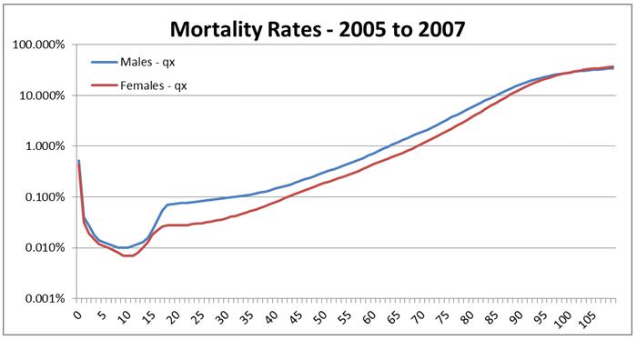
Mortality tables are produced by the AGA and are based on observed mortality outcomes. The key data produced for mortality calculations is the mortality rate (actuaries label this ‘qx’) which represents the probability of a person dying at a particular age in their life. Chart 1 below illustrates male and female mortality rates (please note the altered, logarithmic scale of the vertical axis). For example, there is about a 10% chance that an Australian male will die at the age of 85.
Chart 1: Australian mortality rates by age

An easy way to understand this chart is to note that your chances of dying in any year of your life do not rise above 1% until you are over 60 years old.
If we were sure these mortality rates would remain fixed into the future, meaning there was no trend to improve and no systematic mortality risk of deviating from the trend, then we are left with idiosyncratic mortality, or the randomness of age of death given known mortality rates.
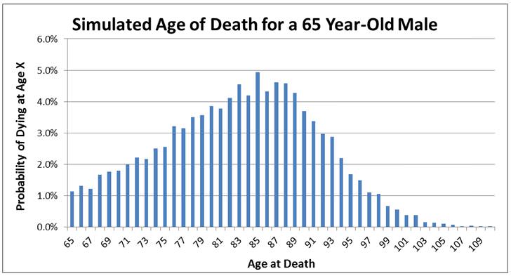
We can get a handle on this risk through simulation. Chart 2 below summarises the results from 10,000 simulations, presenting the likelihood of dying at a particular age for a random male currently aged 65.
Chart 2 is most notable for the breadth of possible outcomes, and the shape of the distribution is not symmetrical and far more spread out than a normal distribution. Regardless of whether the average mortality rate improves (lengthens) or not, we are all exposed to idiosyncratic (or individual) mortality risk.
Chart 2: Summary of 10,000 simulations of the age of death for a male currently aged 65.

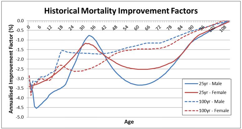
However, systematic mortality risk, excuse the pun, appears alive and well. Historically mortality rates have improved over the very long term (100 years) and over shorter timeframes (25 years). There is evidence suggesting that over very short timeframes (the last three years) there has been continued improvement in mortality rates, a trend highly likely to continue. An historical mortality improvement rate exists for each age and represents the annualised percentage change in the likelihood of dying at that particular age. Historical improvement factors are displayed in the chart below:
Chart 3: Historical mortality improvement factors.

A negative number represents mortality improvement (that is, a reduced chance of dying at a particular age). We see that the largest improvement in mortality rates has been for the very young. We also have large improvement factors for ages 55 – 75 over the last 25 years, largely due to medical improvements for diseases such as cancer. The way mortality improvement factors are applied is relatively straightforward. Say the mortality rate (the chance of dying) at a particular age is 5%. Any improvement factor will simply be applied to this rate. So an improvement factor of -1% would mean that the mortality rate in one year’s time would be approximately 4.95% (5% x (100%-1%)) and this effect would compound through time. The upshot is that these negative improvement factors reduce our chances of dying at a specific age.
We don’t know what mortality improvements there will be in the future, as they will be affected by factors such as medical developments, government spending on health and education, changes to standards of living, lifestyle (such as expanding obesity). This creates the systematic mortality risk. The AGA calculates average life expectancy given how different historical (25 year and 100 year) Improvement Factors (IF) continue into the future. Their results are:
Table 2: Life expectancy for a 65 year old if historical improvement factors (IF) continue.
| |
Male |
Male |
Female |
Female |
| |
25 year IF’s |
100 year IF’s |
25 year IF’s |
100 year IF’s |
| 2006 |
85.6 |
84.4 |
88.5 |
87.7 |
| 2010 |
86.3 |
84.7 |
89 |
88 |
| 2020 |
87.9 |
85.3 |
90.2 |
88.7 |
| 2030 |
89.4 |
86 |
91.4 |
89.4 |
| 2040 |
90.8 |
86.7 |
92.4 |
90 |
| 2050 |
92 |
87.3 |
93.3 |
90.7 |
Life expectancy increases as mortality rates improve
So here’s the main issue we are facing. There are plausible scenarios where the life expectancy of those who make it to 65 in 2050 will be 92 for males and 93 for females. Males who turned 65 in 2010 can expect to live to 84.7 if improvements continue at the 100 year average or to 86.3 if they continue at the 25 year average. A male who is 65 in 2050 would need to expect to make their retirement savings last nearly 50% longer (27 years versus 18.5 years). You can clearly see why governments around the world are implementing policies to push back retirement age.
That is it for the introduction. If you were making study notes for Mortality 101, I would suggest:
- it is conditional expectation (how long we expect to live given we make it to 65) which really matters when we are thinking about longevity risk
- idiosyncratic mortality risk represents the individual’s randomness of outcomes given an environment of known general mortality rates. The dispersion of individual outcomes across the population is very large
- systematic mortality risk arises from uncertainty about the average improvement in population life expectancy. If historical mortality rate improvement factors persevere into the future then retirees are facing a scenario of having to make their retirement savings last much longer. And let us not forget the pressures this would place on funding the age pension for longer.
I apologise for the complex jargon. They sometimes quip that actuaries missed the first six years of school when all the other kids were learning short words. While it is easy to poke fun at actuaries, the role they play in understanding, measuring and managing mortality risk is crucial.
It is unfortunate that most people in the industry (super funds and financial planners) spend much more time considering and modelling investment risk than they do mortality risk.
David Bell would like to thank Associate Professor Anthony Asher from University of New South Wales for his assistance with this article.